Clustering

UBUMonitor includes the feature to apply clustering or unsupervised grouping of students (and teachers), based on data collected from logs, grades and activity completion.

Given the complexity of this section and the concepts used, its use is recommended for advanced users with some backgorund in the field. It is also recommended to review the concept of clustering before using this tab.

As with the other tabs, operation is conditional on the prior selection of users, records (in its four variants of component, event, section or module), rating elements and activity completion.

The main window of the clustering feature is shown below.

Clustering main window

The different types of clustering included in this module, partitional and hierarchical, are described below.

Partitional

The first type of clustering available is partitional clustering. Instances (students or teachers) are partitioned into clusters according to their selected data.

In the top left corner you can select the specific clustering algorithm to be applied. Algorithms from two different libraries are included:

• Apache Math algorithms: documentation can be found online at Machine Learning. These are the algorithms included:

  • KMeans++

  • Fuzzy-KMeans

  • DBSCAN

  • Multi-KMeans

• SMILE algorithms: documentation is available online at Smile - Statistical Machine Intelligence and Learning Engine. These are the algorithms included:

  • K-Means

  • X-Means

  • G-Means

  • DBSCAN

Partitional clustering algorithms.

Depending on the algorithm selected, different parameters to adjust are shown on the right. These parameters are different for each algorithm.

Configuration options for partitional clustering

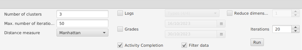
Once the algorithm has been selected and its particular parameters have been set, it is very important to indicate which data you want to use. It is mandatory to tick at least one of the posible options.

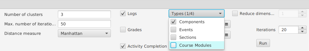
• Logs. Within logs you can also indicate the following:

  • Components

  • Events

  • Section

  • Course models

• Grades

• Activity completion

If no data type has been selected an error message is displayed. It is crucial to confirm the specific data type on which clustering will be performed.

Data selection

If you want to exclude from the analysis those features with constant values for all instances, you will select the Filter data option (it is selected by default). If you also want to reduce the dimensionality of the input set, you will activate the "Reduce dimensionality" option, indicating the number of features to reduce (PCA is applied to reduce the dimension of the input set, although it reduces execution times, it may result in a loss of clustering quality).

Since many algorithms have a random character in their initialization, yo can indicate the number of iterations to be performed. The algorithm will be therefore run the specified number of times, keeping the best result (based on its silhouette analysis).

The last values to be set defines a specific time view to perform the clustering, by indicating the start and end dates for data filtering.

Due to the fact that clustering is unsupervised, and the need of some algorithms to manually suggest the number of groupings or clusters, two methods of inferring the ideal value are provided. However, they are still just suggested values.

The elbow plot and the silhouette value analysis are provided. By choosing one of the two methods from the drop-down and pressing the Analyze button, the corresponding plot is generated for the maximum number of clusters chosen in the slider.

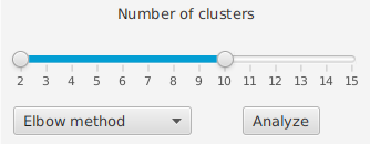
Suggested number of groupings or clusters

The following example shows the elbow plot.

Example of an Elbow plot

Once the algorithm has been executed, and all the previous options have been configured, clicking the Run button will perform the clustering, visualizing the 2D point cloud projection in the 2D Graph sub-tab. The color assigned to the cluster are indicated in the legend together with the cluster number and the number of instances assigned to that cluster. Additionally, the centroids of each cluster are colored in black in the graph.

On the right side of the generated graph, the classified instances are displayed, showing their photo, last name, first name, and assigned cluster number. If you select the Clusters dropdown at the top, you can select and filter only the specific clusters you want to display.

2D Clustering

You can also view the result in a 3D representation of the previously obtained clustering in the 3D graph sub-tab.

3D Clustering

To check the correctness of the executed clustering, indicators are displayed in the Silhouette analysis sub-tab. In this graph, the suitability of the assigned cluster to each instance is represented on a scale of [-1,1]. A value of 1 is an ideal maximum value. In practice, this value will fluctuate between [0,1], indicating whether the instance is poorly or well assigned to that cluster. Negative values indicate that the instance is definitely in the wrong cluster.

Silhouette analysis

Once an appropriate clustering is obtained through the exploratory configuration of the previous options, you can rename the assigned numeric labels. These new text labels are updated dynamically in the generated graphs. This is important if you want to export the data, assigning clusters with more meaningful names than the initial numbers. Once you have finished labeling, by clicking the Export CSV button, you can generate a file with the clustering data for further post-analysis with other tools.

Example of Cluster Labeling

As you add labels, you are allowed limited management of them in the Manage labels sub-tab.

Label Management

Finally, if we have also selected grading elements in the grader's view, additional columns will be added to the right of the results view, displaying grades on a scale of [0,100] (color-coding in red, yellow, green, or purple from worst to best grades), helping to identify and suggest labeling for the instances. If we check the Export grades box, this data will be appended to the CSV export.

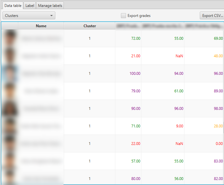
Result of partitional clustering with grading data

Hierarchical

Hierarchical clustering uses a bottom-up approach. Each instance starts in its own cluster and pairs clusters by moving them up the hierarchy.

Hierarchical Clustering Window

To perform these clusters, it uses two configurable parameters:

• Distance Measure

  • Euclidean

  • Mahattan

  • Chebyshov

• Cluster Linkage (distance between clusters)

  • Complete likage

  • Single Linkagee

  • Average Linkage

  • Centroid linkage

  • Ward's linkage

For a more detailed description of these options, refer to the online documentation of its implementation in the SMILE library.

Just like in the partitioning cluster, it is very important to specify which data you want to use. It is mandatory to select at least one of the options.

• Logs. Within logs, you can also specify the data type to be used.

  • Components

  • Events

  • Section

  • Course Modules

• Grades

• Activity Completion

If no data type has been selected an error message is displayed. It is crucial to confirm the specific data on which clustering will be performed.

The last set of parameters to configure includes the start and end dates for data filtering, enabling you to perform clustering on a specific time window within the data.

Once all parameters are configured and data is selected, press the Run button to perform the clustering. In this process, it only generates a visual tree representation called a dendrogram.

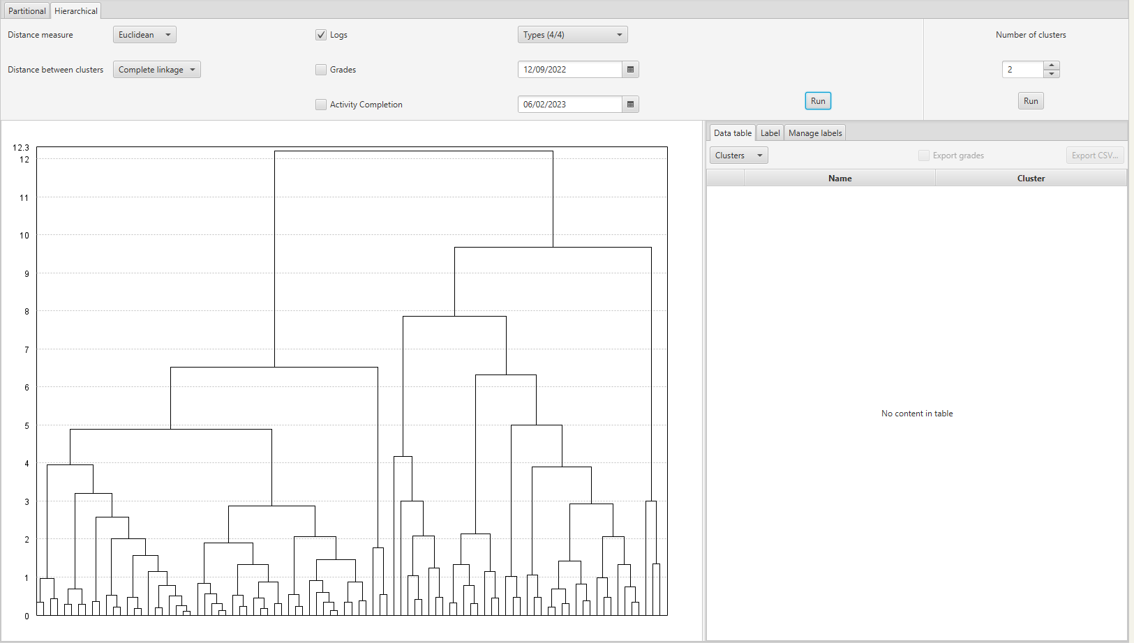
Dendrogram of the Hierarchical Clustering Execution

If you want to generate a specific clustering, you must now select the number of clusters and press the Run button below that number of clusters. This creates a division on the dendrogram, partitioning the instances into the indicated number of clusters. The instances already grouped are displayed on the right, with the same options as in the partitioning cluster.

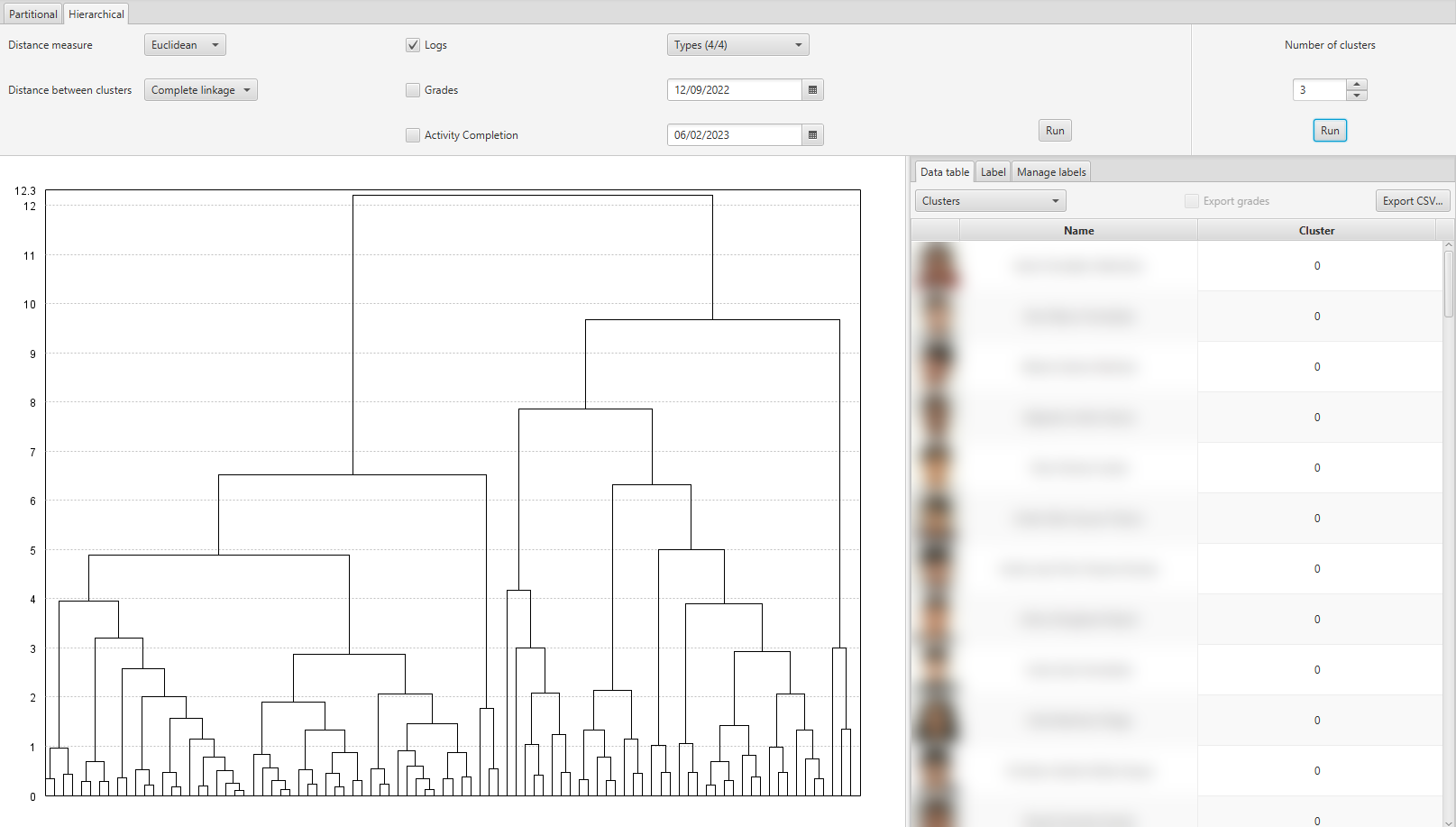
Dendrogram partitioning